Ce tutoriel n’est disponible qu’en anglais…

At first, this post was intended to describe how to manipulate dates with R but, as the idea was coming from the question of one of my students who wanted to analyze his SMS, I thought that I might as well also explain the whole analysis process…

Using my new smartphone (that I started to use on June, 9th) and the apps SMS to text, I have extracted my SMS as a txt file (thank you, Nicolas, I wouldn’t even have had the idea of this post without you ^^). The file (where names were replaced by numbers, phone numbers deleted and message replaced by the number of characters of the sms by using sapply(...,nchar)) is available here (the file is named nv2_sms.txt). Also, Nicolas kindly provided me a sample of his own file, coming from an iPhone (to show different types of date format); the file is available here (and is named nae_sms.txt).

Importing the data into R

Data are imported by:

nv2.sms = read.table("nv2_sms.txt",header=F,sep="\t",stringsAsFactors=F)
names(nv2.sms) = c("date","hour","type","name","nchar")
nv2.sms$name = factor(nv2.sms$name)
nv2.sms$type = factor(nv2.sms$type)

nae.sms = read.table("nae_sms.csv",sep=",",header=T,row.names=1,stringsAsFactors=F)

Who am I texting with?

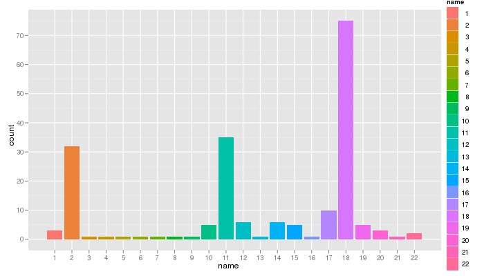
Using the ggplot2 package, I was able to display the number of SMS exchanged with each contact (contacts’ names were removed and replaced by numbers):

qplot(name, data=nv2.sms, geom="bar", fill=name)

and even to check if these messages were sent or received:

qplot(name, data=nv2.sms, geom="bar", fill=type)

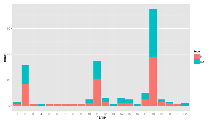
From these charts, are you able to guess which number is my husband, my mum, my sister, my friends, my colleagues, my students…? (if someone finds the first three of the previous list from the first guess, I promise a bottle of good wine, sent anywhere on earth)

To the point: manipulating dates

In my data, the dates are separated into two variables, nv2.sms$date and nv2.sms$hour. The first one is the day, month and year as in “2012-07-07” and the second one is the hour, minute and second as in “17:39:48”. The following lines concatenate both variables into a single one and use the function strptime to convert the result in a full date:

nv2.sms$fulldate = paste(nv2.sms$date,nv2.sms$hour,sep=", ")
nv2.sms$datePX = strptime(nv2.sms$fulldate,format="%Y-%m-%d, %H:%M:%S")

Then, any information can be extracted from the variable datePX with the function format as, for instance, the day of the week or the hour:

nv2.sms$weekday = format(as.POSIXlt(nv2.sms$datePX,origin="1970-01-01", tz="UTC"),"%A")
nv2.sms$weekday = ordered(nv2.sms$weekday,c("lundi","mardi","mercredi","jeudi","vendredi","samedi","dimanche"))
qplot(weekday, data=nv2.sms, geom="bar", fill=weekday)
nv2.sms$hour

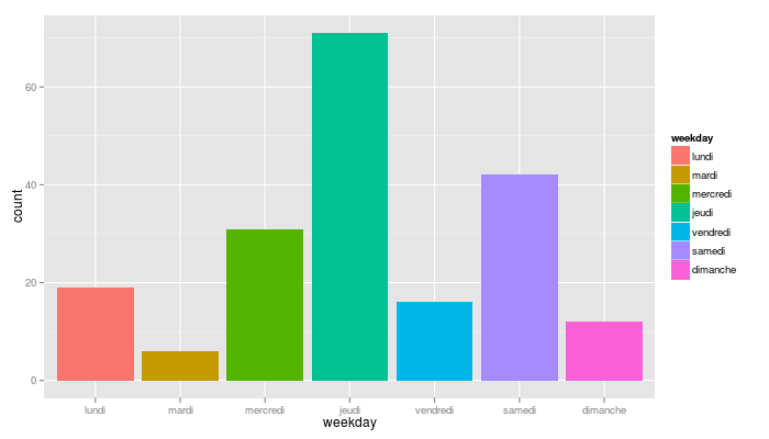
… where I learnt that I like texting on Thursday (can you guess why?)

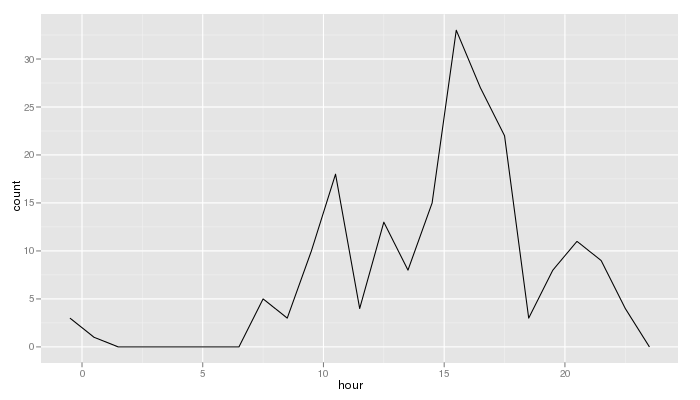
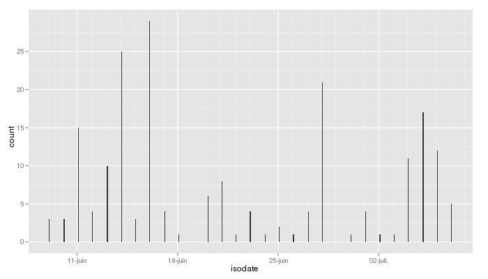
The following command lines will help you display the evolution of your texting activity day by day. Each sms is linked to its day/month/year (the hour is set to 00:00:00 for all messages):

nv2.sms$year = format(as.POSIXlt(nv2.sms$datePX,origin="1970-01-01", tz="UTC"),"%Y")
nv2.sms$month = format(as.POSIXlt(nv2.sms$datePX,origin="1970-01-01", tz="UTC"),"%m")
nv2.sms$day = format(as.POSIXlt(nv2.sms$datePX,origin="1970-01-01", tz="UTC"),"%d")
nv2.sms$isodate = ISOdate(nv2.sms$year,nv2.sms$month,nv2.sms$day,"00","00","00")
qplot(isodate,data=nv2.sms,binwidth=5000)

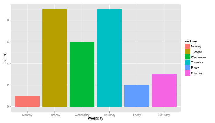
In Nicolas’ data, the dates are included in the variable timestamp which looks like “Jul 28, 2010 6:36:04 PM”. Once again, the function strptime can be used to convert them into a proper date. Unfortunatly, dates are written by month name in English and my locale is… “fr_FR.utf8”!! (this is one of the wonderful things of working with data coming from an American… :-\ ). Setting the locale before the function solves the problem:

Sys.setlocale("LC_TIME","C")
nae.sms$datePX = strptime(nae.sms$timestamp, format="%b %d, %Y %I:%M:%S %p")
nae.sms$weekday = format(as.POSIXlt(nae.sms$datePX,origin="1970-01-01", tz="UTC"),"%A")
nae.sms$weekday = ordered(nae.sms$weekday,c("Monday","Tuesday","Wednesday","Thursday","Friday","Saturday","Sunday"))
qplot(weekday, data=nae.sms, geom="bar", fill=weekday)

The program of the first R meeting that will be held in Bordeaux (France), on July 2nd and 3rd, is now available at http://r2012.bordeaux.inria.fr/programme.html. It includes special sessions about mixed models, visualization, classification, data mining, bioinformatics… Registrations are opened at http://r2012.bordeaux.inria.fr/inscription.html.

PostfixAdmin permet à chaque utilisateur du serveur mail de gérer les réponses automatiques via l’interface utilisateur de postfixadmin. Ce tutoriel explique comment installer cette fonctionnalité (Ubuntu server, 10.04 LTS).

Tout d’abord, un certain nombre de packages supplémentaires doivent être installés :

sudo apt-get install libmail-sender-perl libdbd-mysql-perl libemail-valid-perl libmime-perl
  liblog-log4perl-perl liblog-dispatch-perl libgetopt-argvfile-perl libmime-charset-perl
  libmime-encwords-perl

Attention ! Un utilisateur de Ubuntu server 14.04 (merci Thomas !) me rapporte qu’il a dû aussi installer les packages libmime-encwords-perl, liblog-log4perl-perl, liblog-dispatch-perl pour que l’installation fonctionne correctement.

Ensuite, on crée un utilisateur et un groupe pour gérer le système de vacances ; on affecte un répertoire utilisateur /var/spool/vacation à cet utilisateur :

sudo mkdir /var/spool/vacation
sudo groupadd vacation
sudo useradd -g vacation -d /var/spool/vacation -s /sbin/nologin vacation

Le module de vacation est inclus dans un des répertoire de postfix, éventuellement compressé : il faut le décompresser, le copier dans le répertoire précédemment créé et donner les droits à l’utilisateur vacation sur ce répertoire.

cd /usr/share/doc/postfixadmin/examples/VIRTUAL_VACATION
gunzip vacation.pl.gz
cp vacation.pl vacation.pl.save
cd ..
cp -a VIRTUAL_VACATION /usr/share/postfixadmin/.
cp vacation.pl /var/spool/vacation/.
cd /var/spool/
chown -R vacation:vacation vacation
chmod -R 700 vacation

On édite alors le fichier /var/spool/vacation/vacation.pl pour configurer les paramètres :

our $db_type = 'mysql';
# leave empty for connection via UNIX socket
our $db_host = '';
# connection details
our $db_username = 'postfixadmindb';
our $db_password = 'passwd';
our $db_name     = 'postfixadminuser';
our $vacation_domain = 'autoreply.nathalievialaneix.eu';
# smtp server used to send vacation e-mails
our $smtp_server = 'localhost';
our $smtp_server_port = 25;
# SMTP authentication protocol used for sending.
# Can be 'PLAIN', 'LOGIN', 'CRAM-MD5' or 'NTLM'
# Leave it blank if you don't use authentification
our $smtp_auth = '';
# username used to login to the server
our $smtp_authid = '';
# password used to login to the server
our $smtp_authpwd = '';

où les paramètres doivent être adaptés à votre serveur, et on le rend exécutable :

chmod +x vacation.pl

On met alors à jour le fichier de configuration de postfixadmin : /var/www/postfixadmin/config.inc.php

$CONF['vacation'] = ‘YES’;
$CONF['vacation_domain'] = ‘autoreply.nathalievialaneix.eu’;

Puis on reconfigure postfix : /etc/postfix/master.cf en y ajoutant la ligne suivante vers la fin du fichier :

vacation unix – n n – - pipe flags=Rq user=vacation argv=/var/spool/vacation/vacation.pl -f
  ${sender} ${recipient}

et /etc/postfix/main.cf

transport_maps = hash:/etc/postfix/transport

puis, finalement, en créant un fichier /etc/postfix/transport contenant

autoreply.nathalievialaneix.eu vacation

Les changements sont pris en compte dans postfix avec :

sudo postmap /etc/postfix/transport
sudo /etc/init.d/postfix reload

… et c’est parti pour les vacances !!!

In this post, I give a very simple trick to understand the way a package is organized, which functions are included in and how these functions depend from each others. The idea has been brought by one of my student, Soraya, who is currently working in a very hostile environment, surrounded by true geeks. However, she handles the situation pretty well and manages to take the best from them. As I asked her to insert in her report a chart representing the dependency structure between her functions, she learned from them that tools existed to produce such charts automatically and was able (thanks to R blogger) to find one in an R package.

Suppose that you want to know which functions are included in the package GeneNet (that is of interest for another of my students) and to understand the dependency structure between these functions. First, download the package source, decompress it and use the subdirectory R as the working directory of your R session. If you’re on linux, the following command lines will do the job:

tar zxvf GeneNet_1.2.5.tar.gz
cd GeneNet/R
R

Then, collect and source all files located in this subdirectory and use the function foodweb (from the package mvbutils) to display the dependency structure between functions in this package:

thefiles = list.files()
sapply(thefiles,source)
library(mvbutils)
par(mar=rep(0.1,4))
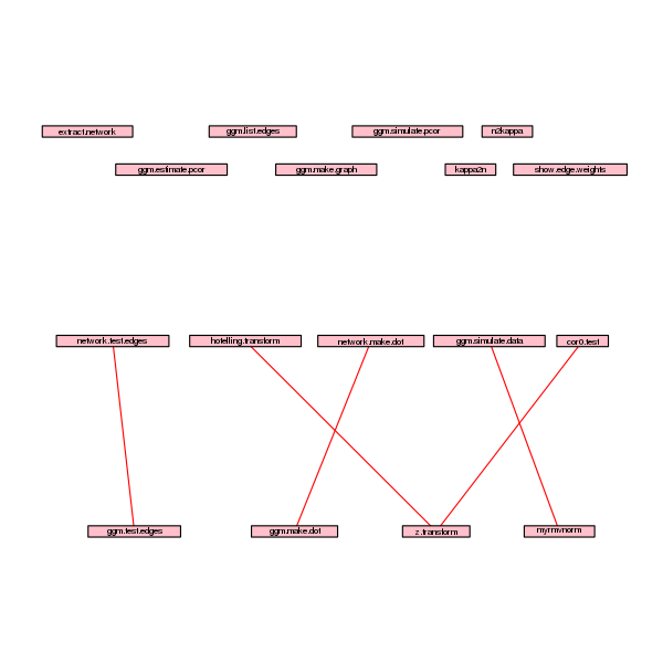
foodweb(border=TRUE,boxcolor="pink",lwd=1.5,cex=0.8)

which gives the following picture:

To spare my student’s time, I did the same with simone

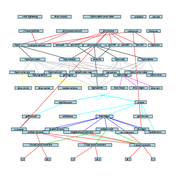
and igraph for which I had to exclude a configuration file:

thefiles = setdiff(list.files(),"config.R.in")
sapply(thefiles,source)
library(mvbutils)
par(mar=rep(0.1,4))
foodweb(border=TRUE,boxcolor="lightgreen",lwd=1.5,cex=0.8)

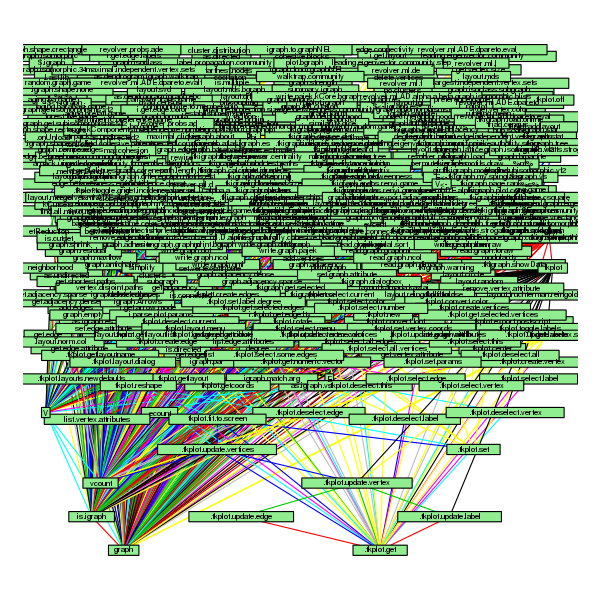
I’m not sure whether the last one is very useful 😉

Now, Soraya is just waiting for her “warhol-R-rabbit” that Paul has promised her to include in her report. It’s gonna be a pop art variant of:

I’m really looking forward to post the R script for it!

Dans ce tutoriel, je me place dans le cadre où j’ai un certain nombre de fichiers de données de structure similaire que je veux traiter à l’aide d’une fonction R qui produira en sortie des graphiques au format png ou n’importe quelle sortie de type « fichier ». J’explique ici comment faire en sorte que les fichiers produits par la fonction soient enregistrés automatiquement dans le même répertoire que le fichier de données d’origine choisi par l’utilisateur et comment personnaliser leurs noms.

Je remercie Soraya avec qui j’ai regardé ce problème durant son stage et qui a fourni une partie de la réponse…

In this post, I want to address the following issue: several data files with a common trame have to be dealt with by an R function. The function should export files (such as images or data files or any other file type). I explain how to create filenames such that the function automatically exports files in the same directory than the input file chosen by the user and how to customize the names of the exported files.
In this post, I want to address the following issue: several data files with a common trame have to be dealt with by an R function. The function should export files (such as images or data files or any other file type). I explain how to create filenames such that the function automatically exports files in the same directory than the input file chosen by the user and how to customize the names of the exported files.

I thank Soraya with whom I’ve been looking at this problem (during her work placement) and who helps me find the answer (especially by pointing out the use of the function file.choose).

Suppose that the following file (it is the famous iris data set):

The following function can be used to make the user chose a data set (that can be this data set but any other one also)

selectFile = function(){
	file = file.choose()
	file
}

Then, start the function by making the user select the original data set. The function then load the data set and grepexpr, substr and paste are used to create new filename as described above:

extractNum = function(){
	# Make the user choose a file
	filename = selectFile()
	# Load the file
	d = read.table(filename,header=T)
	# Select numerical variables
	# (on the basis of the first observation only: might be improved)
	index.num = is.numeric(d[1,])
	# Create new data set with only the numerical variables
	new.d = d[,index.num]
	# Extract from "filename" the pattern to export the new data set
	# (that is, everything before the final dot)
	pat = grepexpr("[.]",filename,grep=F)
	# (in our example, pat is 28 because 28 is the only dot in filename)
	pat = substr(filename,1,max(pat[[1]])-1)
	# (in our example, pat is then /home/tuxette/data1/ex-data)

	# Save the data in Rdata and csv formats at home/tuxette/data1/ex-data-num.Rdata
	# and home/tuxette/data1/ex-data-num.csv
	save(new.d,file=paste(pat,"-num.Rdata",sep=""))
	write.table(new.d,file=paste(pat,"-num.csv",sep=""),row.names=F)
}

In this file, note that the dot (pattern argument in the function grepexpr) is a rationnal expression that has to be specified by “[.]” and not only “.”. Then just use:

extractNum()

Write the link to the data set /home/tuxette/data1/ex-data.txt and you should obtain two files with the numerical variables from the iris data set in the original directory of ex-data.txt. Does it work? À suivre… (mais vous pouvez regarder la version anglaise)