For pedagogical purposes, I needed to install rmr2, which is an R package designed to perform mapreduce code in R. This package is part of the RHadoop project which aims at allowing users to manage and analyze data with Hadoop in R. I followed two strategies:

• the first one (not shown in this tutorial) consisted in installing a virtual linux machine (XUbuntu OS) with a one-cluster Hadoop installation on it;
• the second one, which is the topic of this tutorial consisted in installing rmr2 without Hadoop on various OS. This strategy (and its results) is explained in the following.

Overview of the tutorial:

1. Installation with linux
2. Installation with windows
3. Installation with Mac OS
4. Your first mapreduce job

Make it easy: linux…

Installation on linux went smoothly. My system is made of:

• KUbuntu 12.04 LTS
• R is installed through a CRAN repository and updated packages for my distribution can be installed by RutteR ppa as explained in this previous post .

From here, everything is just straightforward:

1. the dependencies are installed starting R and running the command:

   install.packages(c("Rcpp","RJSONIO","bitops","digest","functional","reshape2","stringr","plyr","caTools"))

   or using the sudo apt-get install r-cran-*** command lines for packages *** that are available in the RutteR repositories (note that caTools version was too old in the RutteR repository and that I had to install the package directly from CRAN.</li>

2. then go on this page and pick up the latest built rmr package (for me, it was rmr-3.1.1) and run the command line (in a terminal, not in R):

   R CMD INSTALL rmr2_3.1.1.tar.gz

   which should work properly.

</ol>

You can finally test your installation by starting R and running:

library(rmr2)

Additionally, I provide a use case example to test mapreduce commands in R, at the end of this tutorial.

A nightmarish installation… Windows

Installation on windows was a lot trickier¹, for one because I was using a Virtual Machine and also because… well… windows (what else?). Luckily, thanks to this tutorial, you should be able to avoid most of the troubles I’ve encountered.

64bit installation: easy!

If you are running R on a 64bit Windows (64bit-Windows 7, with the latest R release, 3.1.0), everything should be easy. You just have to:

1. run 64bit version of R and install the dependencies:

   install.packages(c("Rcpp","RJSONIO","bitops","digest","functional","reshape2","stringr","plyr","caTools"))

2. download the Windows built at this link and use the menu “Packages / Install package(s) from zip file” in R.

I hear you say: “easy! So why are you so grumpy about Windows?” Because, I did not want to spoil my computer installing the OS and I thus used a Windows virtual machine through virtualbox. My original VM was a 32bit Windows (see the next section) on which I was not able to install rmr2. While trying to set up a new 64bit Windows VM, I had a message saying me that VT-x was not enabled on my system and I was not able to install windows in virtualbox. More precisely, while starting the installation of Windows, I got the following error:

VT-x/AMD-V hardware acceleration has been enabled,
 but is not operational. Your 64-bit guest will
 fail to detect a 64-bit CPU and will not be able
 to boot. Please ensure that you have enabled
 VT-x/AMD-V properly in the BIOS of your host
 computer.

It took me a while to figure out that I should restart my Ubuntu OS (the host OS, on which virtualbox is running) and enter my computer’s BIOS (for me, press Echap before startup and then F10): you must search for an option (checkbox) saying “Virtualization (VT-x)” and tick it before you start your computer again: this will allow you to install a 64bit OS in virtualbox.

32bit installation: forget it!

If you have a 32bit Windows installation, you should probably forget to install rmr2. The main reason is that the built package available on this page is a 64-bit built. If you install it on Windows 32bit (I personally had a 32bit Windows XP virtually installed with virtualbox on my computer), you will probably succeed the installation and certainly have the following error message whilst trying to load the package into R:

Error: package ‘rmr2’ is not installed for 'arch = i386'

… and “that simple message stopped you?” are you wondering… hell no! Of course, I did try to install it from source using the following steps:

1. I first installed a proper building environment using Christophe Genolini’s tutorial (see section “Configuration de votre ordinateur”; yes, sorry, it’s in French…) which explains how to compile an R  package in Windows (even if why anybody would want to build an R package in Windows was long a mystery for me…);
2. because I still had an error saying g++: unknown command, and then because, the g++ compiler proposed in Christophe Genolini’s tutorial still leads to an error while compiling, I also followed this post to install g++, even though the Path environment variable wouldn’t update using the instructions, I added the following line to the Rpath file (Rpath is the script loading the different programs needed to compile the package as explained in Christophe Genolini’s tutorial):

   set Path=%PATH%;C:\cygnus\cygwin-b20\H-i586-cygwin32\bin

   to set it instead;</li>

3. I downloaded the pkg directory from the rmr2 github directory (for that I used git on linux);
4. and I finally used the standard command lines used to build and install an R  package in Windows:

   C:\Rpath
   R CMD build pkg
   R CMD INSTALL rmr2_3.2.0.tar.gz

   which ended with:

   * installing to library 'C:/Program Files/R/R-3.0.2/library'
   * installing *source* package 'rmr2' ...
   ** libs
   cygwin warning:
     MS-DOS style path detected: C:/PROGRA~1/R/R-3.0.2/etc/i386/Makeconf
     Preferred POSIX equivalent is: /cygdrive/c/PROGRA~1/R/R-3.0.2/etc/i386/Makecon
   f
     CYGWIN environment variable option "nodosfilewarning" turns off this warning.
     Consult the user's guide for more details about POSIX paths:
       http://cygwin.com/cygwin-ug-net/using.html#using-pathnames
   g++ -m32 -I"C:/PROGRA~1/R/R-3.0.2/include" -DNDEBUG     -I"d:/RCompile/CRANpkg/e
   xtralibs64/local/include"  `C:/PROGRA~1/R/R-3.0.2/bin/Rscript -e "Rcpp:::CxxFlag
   s()"`   -O2 -Wall  -mtune=core2 -c extras.cpp -o extras.o
   In file included from C:\PROGRA~1\R\R-30~1.2\library\Rcpp\include\Rcpp.h:27,
                    from extras.h:18,
                    from extras.cpp:15:
   C:\PROGRA~1\R\R-30~1.2\library\Rcpp\include\RcppCommon.h:64: sstream: No such fi
   le or directory
   In file included from C:\PROGRA~1\R\R-30~1.2\library\Rcpp\include\Rcpp.h:27,
                    from extras.h:18,
                    from extras.cpp:15:
   C:\PROGRA~1\R\R-30~1.2\library\Rcpp\include\RcppCommon.h:76: limits: No such fil
   e or directory
   In file included from C:\PROGRA~1\R\R-30~1.2\library\Rcpp\include\RcppCommon.h:1
   85,
                    from C:\PROGRA~1\R\R-30~1.2\library\Rcpp\include\Rcpp.h:27,
                    from extras.h:18,
                    from extras.cpp:15:
   C:\PROGRA~1\R\R-30~1.2\library\Rcpp\include\Rcpp/iostream/Rstreambuf.h:26: strea
   mbuf: No such file or directory
   In file included from C:\PROGRA~1\R\R-30~1.2\library\Rcpp\include\Rcpp/sugar/sug
   ar.h:28,
                    from C:\PROGRA~1\R\R-30~1.2\library\Rcpp\include\Rcpp.h:68,
                    from extras.h:18,
                    from extras.cpp:15:
   C:\PROGRA~1\R\R-30~1.2\library\Rcpp\include\Rcpp/hash/hash.h:25: inttypes.h: No
   such file or directory
   make: *** [extras.o] Error 1
   ERROR: compilation failed for package 'rmr2'
   * removing 'C:/Program Files/R/R-3.0.2/library/rmr2'
   * restoring previous 'C:/Program Files/R/R-3.0.2/library/rmr2'

   That’s where I stopped. If anybody has a hint, I would be happy to take it.</li> </ol>

   Mac OS: no clue

   Installation on Mac OS is almost as easy as installation on Linux (thank you Elise for sending me the command line):

   1. the dependencies are installed starting R and running the command:

      install.packages(c("Rcpp","RJSONIO","bitops","digest","functional","reshape2","stringr","plyr","caTools"))

   2. then go on this page and pick up the latest built rmr package (for me, it was rmr-3.1.1), start R and run the command line:

      install.packages("rmr2_3.1.1.tar.gz", repos=NULL, type="source")

      after having set the working directory to the directory in which the archive has been downloaded.

   You can finally test your installation by starting R and running:

   library(rmr2)

   Does it work?

   Final step is to check if the installation was successful by running a mapreduce job. Start R and do not forget to tell R that you actually don’t have Hadoop install (or it will complain while trying to run a mapreduce job):

   library(rmr2)
   rmr.options(backend="local")

   Then, you can run the following commands:

   # send groups ID (randomly generated from a binomial) to Hadoop filesystem
   groups = rbinom(32, n = 50, prob = 0.4)
   groups = to.dfs(groups)
   # run a mapreduce job
   ## map: key value is the group id, value is 1
   ## reduce: count the number of observations in each group
   ## then, retrieve it from Hadoop filesystem
   output = from.dfs(mapreduce(input = groups, 
                      map = function(., v) keyval(v, 1), 
                      reduce = function(k, vv)
     keyval(k, length(vv))))
   # print results
   ## keys: group IDs
   ## values: results of reduce job (i.e., frequency)
   data.frame(key=keys(output),val=values(output))

   Further examples of mapreduce jobs can be found on the official RHadoop wiki.

   ---

   ¹ Actually, a real p*** in the a***: it took me half a day, far too much for what this OS deserves but as it seems that a bunch of people, and especially students, are using it, I suppose, it was worth the effort…

   </div>

Ce tutoriel explique comment automatiser une tâche de sauvegarde de répertoires spécifique d’un serveur kimsufi sur le backup FTP d’OVH. Le tutoriel est conçu pour une distribution Ubuntu server 12.04 LTS et fortement inspiré par celui-ci.

L’automatisation de la tâche de sauvegarde utilise le package backup-manager disponible dans les dépôts Ubuntu :

sudo apt-get install backup-manager

Dans un premier temps, vous pouvez laisser les champs remplis tels quels ; vous relancez une configuration plus complète avec :

sudo dpkg-reconfigure backup-manager

Les questions suivantes sont posées :

• Please enter the name of the directory where backup manager will store the generated archives : entrer ici le dossier de stockage sur votre serveur, par exemple /home/save. N’oubliez pas de créer le répertoire correspondant et d’en interdire l’accès en lecture à tout autre personne que le propriétaire (root) :

  sudo mkdir /home/save
  chmod o-rxw /home/save

• owner user of the repository : root
• owner group of the repository : root
• storage format : tar.gz (ou tout autre format que vous pourriez préférer pour la compression des archives)
• CRON frequency : weekly (si une sauvegarde hebdomadaire est suffisante ; sinon, daily pour une sauvegarde journalière)
• follow simulink : no (cette option permet de conserver les liens symboliques dans les archives ; si vous souhaitez effectivement conserver les liens symboliques, choisissez yes)
• archive name format : short (si vous préférez un nommage complet, choisissez long)
• age of kept archives : 10 (c’est le nombre de jours durant lesquels les archives seront conservées)
• directories to archive : entrez ici la liste des dossiers/fichiers que vous souhaitez archiver en les séparant par un espace ; par exemple /home/moi /etc/postfix /etc/hosts
• directories to skip in archives : /home/save (pour ne pas sauvegarder le répertoire d’archives lui-même
• encrypt with gpg : les archives peuvent être cryptées avec une clé GnuPG (voir ce post pour de plus amples informations). Si vous souhaitez crypter les données sauvegardées, choisissez yes ; sinon, no
• enable backup-manager's uploading system? : cette option permet de transférer les fichiers sauvegardés sur l’espace backup FTP fourni par OVH avec les serveurs kimsufi. Répondre yes
• transfer-mode : choisir ftp
• remote host list : entrer l’adresse du backup FTP de votre compte OVH ; celle-ci est du type ftpback-.... On la trouve en activant le backup FTP dans le manager OVH : une fois connecté à son manager, choisir dans le menu de gauche “Service” puis au centre “Backup FTP” ; après activation, le login et le mot de passe ainsi que l’adresse du serveur sont envoyés par email (voir aussi ce post)
• remote host user : votre nom d’utilisateur pour la connexion FTP est également fourni dans le manager. Elle est du type ....kimsufi.com
• remote host password : votre mot de passe pour la connexion FTP
• remote host directory : tapez / à moins que vous ne souhaitiez transférer les archives dans un sous-répertoire particulier, par exemple /sauvekimsufi
• automatic burning : si vous souhaitez créer automatiquement une image DVD à graver ; sinon répondre no

Finalisez la configuration en éditant (en mode super-utilisateur) le fichier de configuration /etc/backup-manager.conf en vérifiant en particulier les lignes

export BM_UPLOAD_FTP_PASSIVE="false"
export BM_UPLOAD_FTP_HOSTS="ftpback-..."

Vous pouvez tester la configuration en lançant en super-utilisateur la commande

sudo backup-manager

Si vous avez programmé la sauvegarde d’un nombre important de dossiers lourds, cette commande peut prendre un moment à s’exécuter. Dans ce cas, je vous conseille l’utilisation du logiciel screen :

sudo apt-get install screen

qui permet de lancer une commande dans un terminal que vous détachez avant de quitter votre session :

screen
sudo backup-manager

La combinaison de touche Ctrl+a suivie de la touche d permet de détacher le terminal screen et la commande

screen -r

de le récupérer. Plus d’informations sur screen sur la documentation ubuntu francophone.

La tâche de sauvegarde est ensuite lancée périodiquement automatiquement grâce au fichier cron /etc/cron.weekly/backup-manager.  

This tutorial provides a few tricks that may be useful if you are an academic and want to manage your website with jekyll. It is a follow-up of this post and it explains how to insert mathematics formula on your pages using LaTeX syntax and how to automatically display a bibliography using a simple BibTeX file.

Insert mathematics formulas

You first need to activate MathJax javascript engine adding the following line in the header of your template (the file _layouts/default.html in this post):

Using kramdown syntax, mathematics formulas are displayed when LaTeX code is delimited by $$ and in-line mathematics formulas are delimited by $. For instance,

$$\frac{x^2}{\sqrt{y+1}}$$

will be displayed as

$$\frac{x^2}{\sqrt{y+1}}.$$

Display a BibTeX file

A BibTeX file can be displayed in a customizable way using jekyll-scholar. First, the plugin is installed (on the local computer and on the server) using

sudo gem install jekyll-scholar

then, the plugin is enabled by creating a file _plugins/ext.rb in your website directory (myWS in the example on this post).

jekyll-scholar is configured by editing the _config.yml file. I added to this file the following lines:

scholar:
  style: assets/bibliography/mycslfile.csl
  locale: en

  sort_by: year
  order: descending

  source: assets/bibliography
  bibliography: mybiblio
  bibliography_template: bibtemplate

  replace_strings: true

  details_dir:    bibliography
  details_layout: bibtex.html
  details_link:   Details

  query: "@*"

This configuration reads:

• the style is provided using a CSL file (XML language) which explains jekyll-scholar how to display one reference using the corresponding BibTeX entry. I am using a personalized CSL file which is adapted to my personal needs from one taken on the official repository. Most standard BibTeX styles (bst files) are available as CSL styles. My personalized CLS file is saved as assets/bibliography/mycslfile.csl;
• my BibTeX file is saved in assets/bibliography in a file named mybiblio.bib. A BibTeX entry is composed of standard BibTeX fields and I added a couple of custom fields to allows a more complex presentation of an entry. For instance:

  @ARTICLE{boulet_etal_N2008,
    author = {Boulet, R. and Jouve, B. and Rossi, F. and Villa, N.},
    title = {Batch kernel {SOM} and related {L}aplacian methods for social network analysis},
    journal = {Neurocomputing},
    year = {2008},
    volume = {71},
    pages = {1257-1273},
    number = {7-9},
    doi = {doi:10.1016/j.neucom.2007.12.026},
    keywords ={self-organizing maps, social network},
    webnote = {Comments upon this article can be found on Nature web site.},
    website = {http://www.elsevier.com/wps/find/journaldescription.cws_home/505628/description}
  }
  @CONFERENCE{rossi_etal_DD2011,
    author = {Rossi, F. and Villa-Vialaneix, N. and Hautefeuille, F.},
    title = {Exploration of a large database of French notarial acts with social network methods},
    booktitle = {Digital Diplomatics 2011},
    year = {2011},
    address = {Napoli, Italy},
    eventdate = {2011-09-29/2011-10-01},
    keywords = {social network},
    poster = {yes},
    website = {http://www.cei.lmu.de/digdipl11/}
  }

  with the custom fields webnote to display additional notes on the webpage, website to display the website of the conference or of the journal, poster (or slide) to indicate that a poster file is associated to this file). Except for the webnote field, all these personalized fields are used in the bibliography template (see below). For the webnote field, it is used directly in the CSL file (see above) in which I have added the following line: </a> which prints webnote in italic.
• Then, the bibliography layout is included in a file _layouts/bibtemplate.html and contains the way jekyll-scholar should mix informations included in the BibTeX entry with the output of the CSL processing. It combines standard HTML with liquid syntax: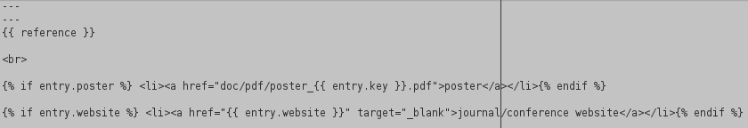 refers to the output of the entry after CLS processing. Then, if a field poster exists in the BibTeX entry, a link is created to the poster, based on the BibTeX key. The field website is processed similarly.

Finally, a file publications.md can be created (using kramdown syntax) in the website directory:

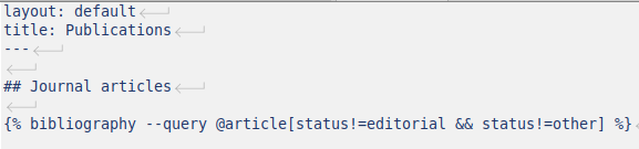
This file indicates to jekyll-scholar that the bibliography must be displayed. Only entries of type @article are selected and those with a BibTeX field status (it is another custom BibTeX field that I have used in some entries) equal to “editorial” or to “other” are filtered out. Using the command

jekyll serve

Jekyll then processes your BibTeX file and you can finally obtain (with some efforts, I must confess) something that looks like this page.

This tutorial explains the main steps to create and manage a static website with jekyll and git.

Requirements: At the begining of the installation, I had

• a desktop computer with Kubuntu 12.04 LTS OS. A local apache server on your computer would also be helpful to test your website locally before sending it to the server;
• a server with Ubuntu server 12.04 LTS and a git server installed.

Overview of this tutorial:

1. Install jekyll
2. Make your first website
3. Use bootstrap css
4. Deploy your website using Git

Install

Jekyll is a static web generator written in ruby. To install it, you first need to install (both on your local computer and on your server), ruby:

sudo apt-get install ruby1.9.1 ruby1.9.1-dev make

Then, using ruby repository you can install jekyll and also kramdown, a ruby library that can convert markdown (markdown is a plain and very simple text formatting syntax that can be converted into HTML).

gem install jekyll
gem install kramdown --no-rdoc --no-ri

On you local computer, create a directory that will contain your website, say myWS then make the first file you need, the configuration file

touch config.yml

An example of configuration file is provided below:

markdown: kramdown
name: "Tuxette Chix"
description: "my website"
url: "http://www.domain-name.org"

Write your first page

This part of the tutorial is partially inspired by this tutorial which helped me a lot to begin. You jekyll website is made of the following directory/files at least (all included in the previously created dirctory myWS:

• a directory _layouts that contains the layout of every pages in your website (you can have different layouts corresponding to different types of pages in your website but at least this directory contains a default layout called, for instance, default.html
• a file index.md that contains the content of your website’s index page. Combined with the chosen layout, it will be converted into a proper html file. Additionally any file md or html file in myWS that begins with the proper syntax (see below) will be converted into a proper html file and added to the website.

Here is a very simple example of what can be done to obtain your first website:

Layout default.html

The part with Your website with Jekyll and Git corresponds to liquid syntax and reads “if a title page has been provided in the processed file, then this title is displayed. Otherwise, nothing is displayed.” Similarly

deb http://cran.univ-paris1.fr/bin/linux/ubuntu precise/

gpg --keyserver keyserver.ubuntu.com --recv-key E084DAB9
gpg -a --export E084DAB9 | sudo apt-key add -
sudo apt-get update
sudo apt-get upgrade
sudo apt-get install r-base-core r-base-dev

sudo add-apt-repository ppa:marutter/rrutter
sudo apt-get update

sudo apt-get install curl

sudo apt-get install r-cran-plyr r-cran-xml r-cran-reshape r-cran-reshape2 r-cran-rmysql

install.packages(c("jpeg","jsonlite","data.table","httr"))

source("http://bioconductor.org/biocLite.R")
biocLite("rhdf5")

conftest.c:1:17: fatal error: jni.h: No such file or directory
compilation terminated.
make: *** [conftest.o] Error 1
Unable to compile a JNI program

File index.md

---
layout: default
title: Welcome!
---
# Welcome on my website

## About me

My name's *tuxette* and there's nothing terribly interesting that I can tell you.

## About my blog

My blog can be seen at (this link)[http://www.domain-name.org].

The file must start with its description surrounded by --- ; the layout that the file will be combined to is default.html and the page is assigned a title “Welcome !”. Then, the content of the file is provided: the syntax used is that of kramdown: # is used to indicate h1 text, ## is for h2 (and so on), *tuxette* displays the text in italic, and hyperlinks are easily included. kramdown syntax can be combined with standard HTML for more specific needs.

Generate your first website

Then, you can generate the website using the command line (inside the directory myWS)

jekyll serve

The website is created in the directory _site and if you have an apache server installed on your computer, you can see it opening the url http://localhost:4000 in your favorite browser. Jekyll server is stopped using Ctrl+C.

Use bootstrap css

Up to now, you website is probably very ugly. You should choose a css to display it nicely. As I am far from having good tastes (as this blog is the proof of), I chose security with bootstrap. There’s a very nice way to personalize bootstrap in jekyll while staying up to date with the development of the css as described at this link (that uses the css generator less) but I was not able to deploy it on my website due to version conflicts. Thus, I opted for the easy way:

• I downloaded bootstrap and copied it in a directory assets/bootstrap in my website’s directory. It contained css files, javascript files and fonts:
• then I updated the file layout.htmlto allow for the use of bootstrap by adding the following header:and the following lines in footer:

Your website should now display much more nicely and you can use all components provided by bootstrap.

Deploy your website with Git

More information on git and gitolite at this page and at the end of this page (sorry, in French…).

There is many ways to deploy your website on your server. The simplest is to generate it locally and then to send the directory _site on your server by FTP. However, if you are familiar with git, you may want to use it to do the job for you: when the git repository is updated, the website is automatically re-generated on your server. Deployment methods are explained on this page and I chose the post-receive approach. To do so,

1. I first created using the git project names mywebsite using the standard config file as explained at the end of this page;
2. then, I created a bare repository in the directory containing git repositories on my server (on Ubuntu 12.04 LTS, using gitolite, this directory is usually /var/lib/gitolite/repositories but you can locate it using locate git otherwise). This command lines are executed being root or git user:

   mkdir mywebsite.git
   cd mywebsite
   git --bare init

3. still on the server, I created a directory that will receive the resulting website:

   mkdir ~/jekyll-website
   chown gitolite:gitolite -R ~/jekyll-website

   (the last lines give rights to gitolite on the directory)</li>

4. then, in /var/lib/gitolite/repositories/mywebsite.git/hooks, I created a file named post-receive that contained instructions to be run when git receives new contents:

   GIT_REPO=/var/lib/gitolite/repositories/mywebsite.git
   TMP_GIT_CLONE=/var/lib/gitolite/tmp
   PUBLIC_WWW=/home/me/jekyll-website
   
   git clone $GIT_REPO $TMP_GIT_CLONE
   jekyll build -s $TMP_GIT_CLONE -d $PUBLIC_WWW
   rm -Rf $TMP_GIT_CLONE
   chmod o+rx -R $PUBLIC_WWW
   exit

5. finally, on my local computer, I created a git repository corresponding to the project mywebsite in the directory myWS using

   git init

   I added all files necessary to deploy the website (hence not the ones included in _site with

   git add _layouts/*.*
   git add index.md
   git add assets/bootstrap

   and pushed them on the server after I have registered the remote repository:

   git remote add public gitolite@domain-name.org:mywebsite.git
   git push public master

</ol>

You’re done. I’ll explain soon how to use jekyll-scholar and BibTeX to automatically generate a publication list from a BibTeX file.

</div>

This post explains how to install all (or at least most of) the R packages described in the MOOC “Getting and Cleaning Data” offered by Johns Hopkins University on the MOOC coursera if you’re using Ubuntu. Moreover, it gives pratical advices for staying up-to-date with your R installation on this OS.

R installation: CRAN repository and RutteR ppa

First of all, the version of R included in Ubuntu repositories may be a bit old. I advice using the official CRAN repository editing (as root) the file /etc/apt/sources.list and adding the following line at its end:

deb http://cran.univ-paris1.fr/bin/linux/ubuntu precise/

adapt the previous line with your favorite CRAN mirror and your distribution’s name) and then

gpg --keyserver keyserver.ubuntu.com --recv-key E084DAB9
gpg -a --export E084DAB9 | sudo apt-key add -
sudo apt-get update
sudo apt-get upgrade
sudo apt-get install r-base-core r-base-dev

Packages for the CRAN repository are built on a Launchpad PPA called RutteR. It is possible to use the PPA itself, which includes a few more packages than the CRAN repository. Installing the PPA is done using:

sudo add-apt-repository ppa:marutter/rrutter
sudo apt-get update

Curl

As explained in the first week videos of the course, data avalaible through an ‘https’ connexion can be downloaded using the option method="curl" in some functions. However, on Ubuntu, you first need curl to be installed:

sudo apt-get install curl

Packages included in the repositories

Some packages are included in the repositories and can be installed directly using the command line:

sudo apt-get install r-cran-plyr r-cran-xml r-cran-reshape r-cran-reshape2 r-cran-rmysql

Packages easily installed from R

Some packages are not available in the RutteR ppa but are nevertheless easily installed in R using the CRAN repositories:

install.packages(c("jpeg","jsonlite","data.table","httr"))

or by the bioconductor project:

source("http://bioconductor.org/biocLite.R")
biocLite("rhdf5")

The hard way: package xlsx

xlsx may be a bit tricky to install because you need rJava which itself requires a proper JVM on your system. A problem has been reported trying to simply install the package r-cran-rjava:

conftest.c:1:17: fatal error: jni.h: No such file or directory
compilation terminated.
make: *** [conftest.o] Error 1
Unable to compile a JNI program

This problem is solved by:

• first installing openjdk version 7:

  sudo apt-get install openjdk-7-*

  The installation is properly registered by your system using

  update-alternatives --config java

  and choosing openjdk-7 as the default JVM.</li>

• rJava can now be installed. Only, java configuration for R is updated before using the ubuntu package:

  sudo R CMD javareconf
  sudo apt-get install r-cran-rjava

• finally, in R, run:

  install.packages("xlsx")

</ul>

Now, you just have to learn how to use all these 😉

</div>